Kernels and the First Isomorphism Theorem
Introduction
One of the most seminal and revolutionary ideas of the 19th century was that of a group, which forms the basis for all subsequent developments in mathematics and science, and is a cornerstone of modern algebra. But this abstraction that allows us to think about and prove results in generality, in essence, draws its strength from three fundamental insights: that of a group homomorphism, a normal subgroup, and the factor group.
In the words of I.N. Herstein:
In a certain sense, the subject of group theory is built up out of three basic concepts, that of a homomorphism, that of a normal subgroup, and that of a factor group of a group by a normal subgroup.
We will explore some of these key insights that make groups a powerful and useful abstraction.
Group Homomorphism
The term homomorphism comes from the Greek words: Homo meaning same and Morphism meaning form. This notion of a group homomorphism was introduced by Camille Jordan in 1870 in his famous book Traité des substitutions and is a natural generalization of the concept of group isomorphism.
Notice that the group operations need not be the same. But what the definition guarantees is that combining elements and mapping them can be done in any order. One consequence of this definition is that the Cayley tables are preserved under this mapping.
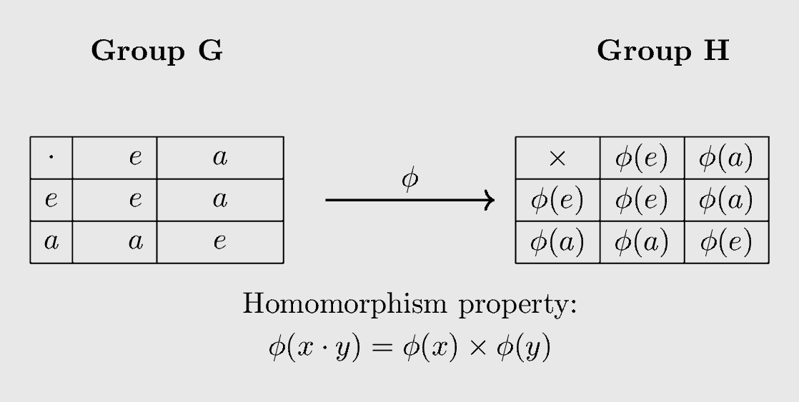
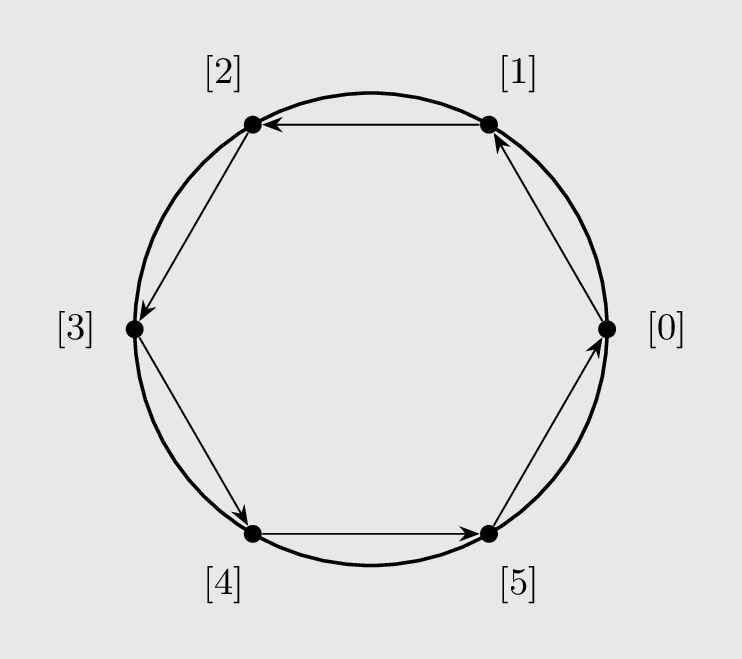
To make the discussion more grounded and concrete, consider the mapping: \(\phi : \mathit{Z} \to \mathit{Z_6}\) defined as $\phi(x) = x \mod 6$. It can easily be verified that it is well-defined and hence a function. Also, notice that
Hence, it is a homomorphism.
A homomorphism, being a map, has a domain and a codomain, $\mathbf{Z}$ and $\mathbf{Z_6}$ in this case. And the image of the homomorphism is a subset of the codomain, which in this case so happens to be the codomain itself. But a homomorphism need not necessarily be surjective, to see why, take the same mapping, but this time define it as $\phi(x) = x \bmod 3$. Now, the image of the homomorphism is a proper subset of the codomain. Furthermore, a homomorphism may or may not be injective. If it so happens that it is both, then we have an isomorphism.
Another important takeaway from this example is the observation that this homomorphism partitions the group of integers (domain) into six distinct equivalence classes, namely $[0],\; [1],\;[2],\;[3],\;[4],\;[5]$, as its image which is something that will come up later and can only be properly understood after much of the discussion has been carried out.
A homomorphism has many properties, most of which can be proved from its definition. But for brevity’s sake, these properties are not being stated here. The interested reader can find them at this link: Properties of a Group Homomorphism.
Kernel
In defining a homomorphism between two groups, there is one subgroup of the domain that is of particular importance, one that deserves its own name, The Kernel of the homomorphism.
Note that the kernel is always a non-empty set given a non-empty domain. To see why, consider:
By right cancellation, we have $\overline{e} = \phi(e)$. And, $\overline{e}$ is the identity of $\overline{G}$.
And now, to show that it is indeed a subgroup of the domain, observe that it is a non-empty subgroup of $G$ containing the identity. So, all we need to prove is if $a, b \in Ker\;\phi$, then $a\cdot b^{-1} \in Ker\;\phi$. And this can be proved as follows.
Hence, $ab^{-1} \in Ker\;\phi$.
The importance of the Kernel comes from the fact that it is a normal subgroup of the group $G$ (domain). And being a normal subgroup, it induces a quotient group $G / Ker\;\phi$, the elements of which form a partition of the original group. So, it causes a systematic collapse of the group into a smaller group while preserving the homomorphism-invariant properties. This is more obvious if we look at the Cayley tables of the original group and the quotient group induced by the kernel, in which each coset of the $Ker\;\phi$ maps to a single element in the quotient group.
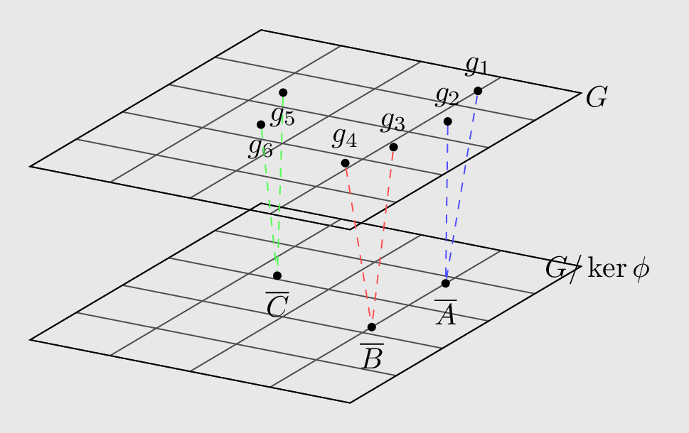
This collapse is n-to-1 based on the order of $Ker\;\phi$. To make this notion more concrete, let’s go back to our previous example and consider the subgroup \(6\mathit{Z} = \{6k \;| k\in Z\}\) of the $\mathit{Z}$ which is normal being a subgroup of an abelian group. This normal subgroup in itself induces a quotient group $\mathit{Z}/6\mathit{Z}$. What is important about this quotient group is its algebraic structure: \(\{6\mathit{Z},\; 1 + 6\mathit{Z},\; 2 + 6\mathit{Z},\; 3 + 6\mathit{Z},\; 4 + 6\mathit{Z},\; 5 + 6\mathit{Z} \}\). It not only partitions the group into six distinct equivalence classes but is also isomorphic to the cyclic group $\mathit{Z_6}$, an elusive but important connection that we will deal with and formalize in the next section, but before that, some proofs and observations are in order.
Proof of the normality of the Kernel
For a subgroup $H$ to be normal in $G$, $xHx^{-1}\subseteq H$ has to hold for all $x \in G$.
To see why this holds for $Ker \;\phi$, consider $gkg^{-1}$ where $g\in G$ and $k \in Ker\;\phi$. What we want to show is that it always belongs to $Ker \;\phi$, that is $\phi(gkg^{-1}) = \overline{e}$. This can be shown as follows:
Hence, $gkg^{-1}\in Ker\;\phi\;\; \forall g\in G$ and $Ker\;\phi$ is normal in G.
The first Isomorphism theorem
This theorem was first stated and proved by Camille Jordan in 1870. It formalizes the connection observed in the example above, highlighting its significance: through a homomorphism we can gain insight into both a group and its quotient, while conversely the quotient group provides a lens into the structure of its homomorphic images.
Proof
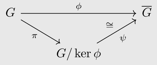
Let us use $\psi$ to denote the correspondence $gKer\;\phi \to \phi(g)$. First, we need to show that this correspondence is well-defined. Observe that,
This argument in reverse can be used to show that this mapping is one-to-one(injective).
For the surjectivity condition, for any $\phi(x)\in Im(G)$, take $xKer\; \phi$ which maps to $\phi(x)$.
And finally, the operation preservation: \(\psi(aKer\;\phi\cdot bKer\;\phi) = \psi(abKer\;\phi) = \phi(ab) = \phi(a)\phi(b) = \psi(aKer\;\phi)\psi( bKer\;\phi)\)
Hence, it is an isomorphism.
Algebraists normally represent this connection through this succinct diagram that captures the essence of the First Isomorphism Theorem in a commutative triangle.
Following this theorem, some important observations are in order. The most obvious one would be that all the homomorphic images of a group can be determined using its quotient groups. This observation can be reformulated in different terms as a theorem in its own right.
This mapping $\gamma : G\to G/N$ is called the natural homomorphism from $G$ to $G/N$, defined as $\gamma(g) = gN$.
Then, we see that the homomorphic images of an abelian group are abelian since all its quotient groups are abelian. Furthermore, the number of homomorphic images of a cyclic group of order n is the number of divisors of n, since there is exactly one subgroup of G (and therefore one quotient group of G) for each divisor of n.
In completion of what was promised earlier, we now have stated enough to be able to explain why a homomorphism partitions a group. By Theorem 2, we know that every normal subgroup is the kernel of a homomorphism, and being normal, it partitions the groups into cosets as a quotient group, which is isomorphic to the image of the homomorphism, the kernel of which is the normal group used to partition the original group.
To make everything concrete, we state another example: Consider the group $GL(2, R)$ and its normal subgroup $SL(2,R)$. The quotient group induced by $SL(2, R)$ partitions the group into distinct cosets of matrices such that all the matrices in a coset have the same determinant, the values of which are the set of real numbers. In terms of homomorphism, this can be restated as $\phi: GL(2, R) \to R^*$ defined as $\phi(A) = detA$, the kernel of which is $SL(2, R)$. So, in short:
Additional Section
This section is for those who have had exposure to linear algebra and have studied elementary linear algebra, but before we state an example explaining how the above-stated discussion is pertinent to linear algebra and linear transformations between vector spaces, we introduce some terminology commonly understood in this context.
In linear algebra, we extend the concept of a group to a space by introducing additional distributive properties and an underlying field. Similarly, subgroups in this context can be viewed as subspaces. As for normal subgroups, we don’t have an explicit terminology for them in this context, since every subspace is normal, being a subspace of an abelian group(Vector space).
The term commonly used for a map in linear algebra is transformation or linear transformation $T : V \to W$, and every transformation is a group homomorphism as it preserves the group operation:
Whilst every invertible transformation is a group isomorphism.
Moving onto the kernel, it is called the kernel of $T$, or if the transformation is represented in matrix form, the null space of $T$, which is the subset of the domain satisfying the equation $Ax = 0$. In contrast, the quotient group induced by the kernel becomes a quotient space induced by any subspace of a vector space. And finally, the first isomorphism theorem becomes: \(V/Ker(T) \cong Im(T)\)
Now that we are done with the basic terminologies, let’s state an example to explain how the above-stated concepts apply to linear algebra.
Consider the transformation $T:\mathbb{R}^3 \to \mathbb{R}^3$ defined as $T(x,\;y,\;z) = (x +2y+3z,\;x +2y+3z,\;x +2y+3z)$, the matrix of which in the standard basis can be represented as:
It is obvious from the matrix representation that this transformation maps $\mathbb{R}^3$ onto the one-dimensional subspace of $\mathbb{R}^3$ spanned by the vector $(1,1,1)$.
And the null space of this matrix is the subspace of $\mathbb{R}^3$ spanned by the vectors $(-2, 1, 0)$ and $(-3, 0, 1)$.
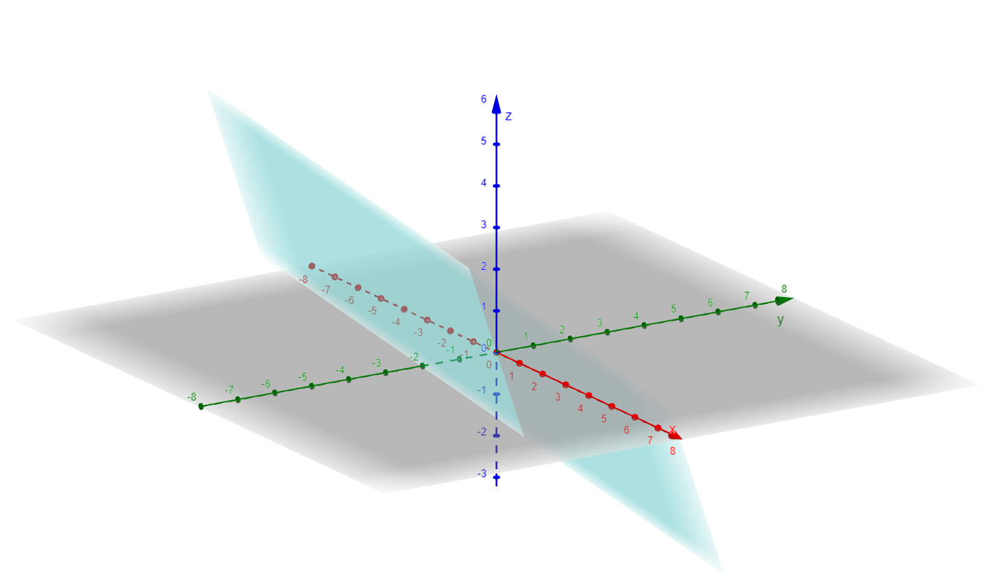
The null space being a subspace of the domain $\mathbb{R}^3$ induces a quotient space $\mathbb{R}^3/Ker(A)$ that partitions the 3-dimensional space into cosets, which can be geometrically thought of as planes parallel to the null space but displaced from the origin by some vector, all of which are the solution sets of vectors belonging to the Image of $T$.
To make this idea more concrete, consider the solution set of the vector $v = (1, 1, 1) \in Im(T)$. In matrix notation, this can be expressed as:
We can solve it either by using Gaussian elimination, or, in our case, simply by observing the fact that $v \in Im(T)$ and that the null space partitions the domain into cosets, which in this case are planes. So, the solution set in this case would simply be the set $w + Ker(T)$ where $w$ is a particular solution of this equation, which can be geometrically expressed as follows:
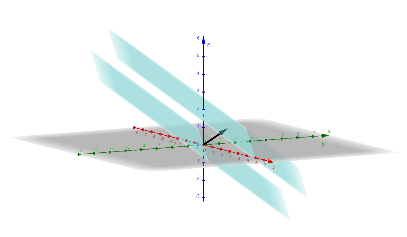
Another way to see why this must be the case is to observe that $A$ is a linear operator, and letting $w$ be a particular solution of the above equation, we see that:
Conclusion
The First Isomorphism Theorem acts as an intermediary in abstract group theory and its practical uses. The theorem untangles kernels, images, and quotient groups by demonstrating the isomorphic structure a group retains and reflects through its homomorphisms. The examples in $Z/6Z \text{ and } GL(2, R)$ serve to showcase the theorem’s power in resolving what appear to be convoluted issues. The comparison to linear algebra also shows the theorem’s wide-ranging impact in mathematics. More than a mere formal outcome, the theorem embodies a crucial idea. When we define one object in terms of another, the part we end up keeping is, in all its redundancy, the group’s core. This understanding goes beyond reshaping algebra. It changes how contemporary mathematics perceives symmetry, structure, and transformation.
References
- Joseph A. Gallian. Contemporary Abstract Algebra, 10th Edition. Cengage Learning, 2016.
- Kenneth Hoffman and Ray Kunze. Linear Algebra, 2nd Edition. Prentice Hall, 1971.